T-distributed Stochastic Neighbor Embedding

State of Art dimensional reduction technique for visualization.

t-SNE stands for T-distributed Stochastic Neighbor Embedding(hard to remember though:< ) developed by Laurens van der Maaten and Geoffrey Hinton. It is non-linear reduction technique which helps in embedding high dimensional data in 2-D or 3-D space for visualization.

Looking at the write-up on Principal Component Analysis, PCA was not doing well except for ‘0’ with the MNIST dataset in 2-D. It was hard to visualize and distinguish between the other numbers. PCA tries to preserve the global structure of data whereas t-SNE preserves local structure too.

Understanding Neighbourhood and Embedding

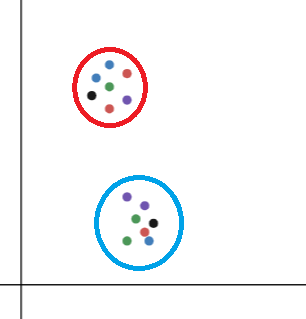
In the above figure, consider a point as x_i in the red cluster. The cluster represents the neighbourhood of x_i(N(x_i)).

N(x_i)={ x_j such that x_i and x_j are geometrically close.

Here, N(x_i) contains all the points present in the red cluster as they are close to x_i.

For every point in higher dimensional space, a new point will be created in the lower dimensional space by preserving the distance between points in the higher dimensional space, known as Embedding.

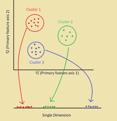
Here, all the points in respective clusters have been embedded on to 1-D space. The intra-cluster distances i.e distance between points in the clusters are same, but inter-cluster distances are not preserved.

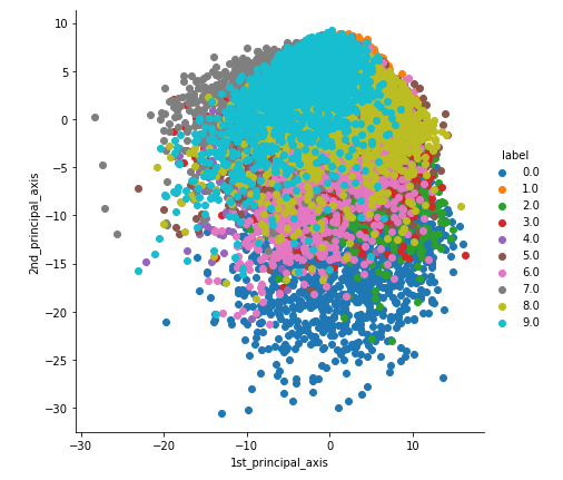
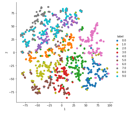
2-D Visualisation of MNIST data

t-SNE is imported from sklearn.manifold.

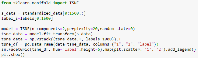
Perplexity defines the number of points closer to the selected point in the neighbourhood. Default iterations size=1000.

With perplexity=20.

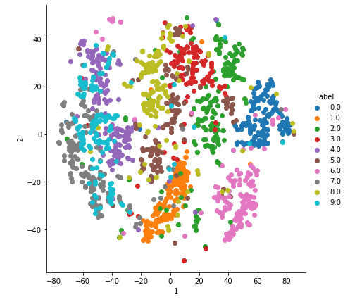
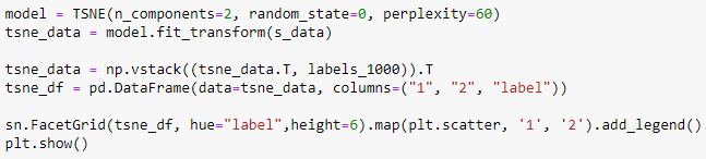
With perplexity=60.

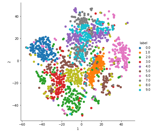
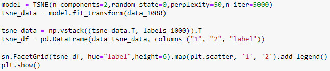
With perplexity=50, iterations=5000.

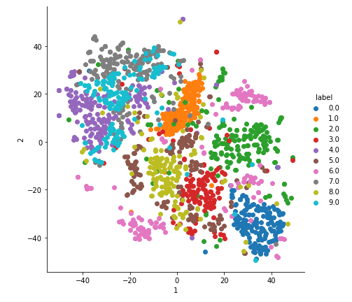
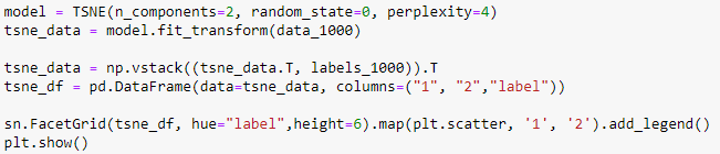
With perplexity=4.

In the above plot, the labels cannot be differentiated as the perplexity is very less.