Ever wondered how to reduce higher dimensional data to a lower-dimensional data to visualize it better?
Possible to interpret this image?
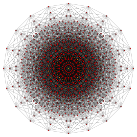
It’s a 10-D cube and it’s hard to visualize this figure.
Humans can only visualize 1D, 2D, and 3D spaces. Even though we live in a 3D world, our eyes can see only in 2D. Our retina has a 2D surface and it’s the 2D projection of 3D objects we are looking at. So, in order to get a clear view of N-dimensional data, one needs to have an (N-1)-dimensional retina surface and would see the N-dimensional objects as (N-1)-dimensional projections. Practically, this ain’t possible.
“Visualize this thing that you want, see it, feel it, believe in it. Make your mental blueprint, and begin to build.” -Robert Collier
Principal Component Analysis generally termed as PCA, is a handy solution for solving the dimensionality problem. Following the above quote by Robert Collier, one has to visualize and understand the data prior to building a model.
PCA helps to remove the features with less variance. Consider a simple example of dataset with only two features. One of the features representing the blackness of hair and the other feature being the weight of an individual. All the data points are from Indians.
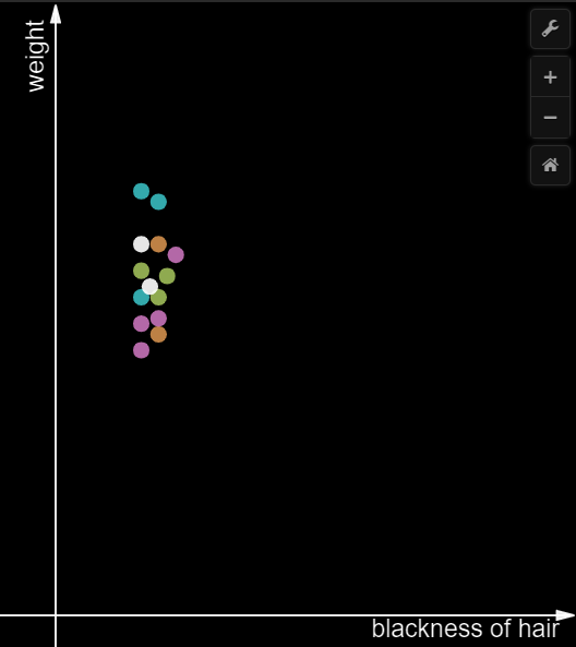
In the above image, the variance over the weight axis is high compared to the variance over the x-axis which is very less. Suppose, the idea is to convert 2D to 1D, then the x-axis can be eliminated. All the points over the y-axis can be plotted on a single axis(1D). Through this way, the direction with maximal variance is preserved without the information being lost.
What if the features are equally distributred over both the axis?
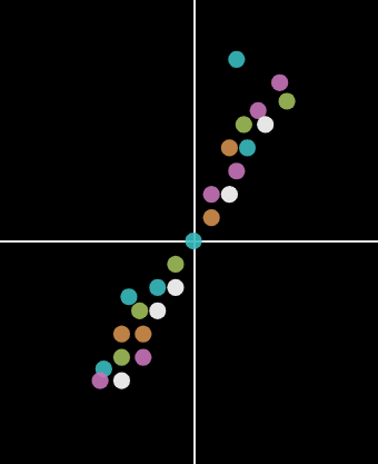
In the above figure, the variance on X-axis and Y-axis is similar. It is not a good idea to eliminate one of the axis in order to reduce it to 1D. Instead draw a straight line(X’) through the points where the variance is high, and a line(Y’) perpendicular to X’.
Dimensionality Reduction of MNIST Data:
Download the dataset from here.
mnist1= pd.read_csv('./mnisttrain.csv')
lab=mnist1['label']
#Drop the label feature in the original dataset
mnist= mnist1.drop("label",axis=1)
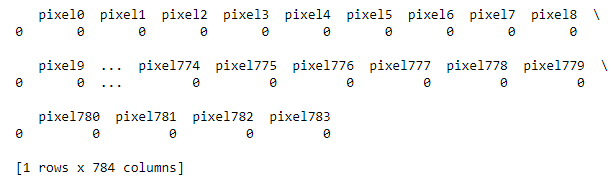
print(mnist.head(1))
Load the mnist data, and remove the labels from the original dataset.
Datapoint with 784 features would look like this:
Use only 20000 points for faster computation, and standardize the data.
from sklearn.preprocessing import StandardScaler
labels=lab.head(20000)
data1=mnist.head(20000)
#standardize the data
standardized_data = StandardScaler().fit_transform(data1)
data=standardized_data
PCA is imported from sklearn.decomposition, considering all the 784 dimensions.
from sklearn import decomposition
pca = decomposition.PCA()
pca.n_components=784
pca_data = pca.fit_transform(data)
percentage_var_explained = pca.explained_variance_ / np.sum(pca.explained_variance_);
cumulative_var_explained = np.cumsum(percentage_var_explained)

plt.figure(1, figsize=(6, 4))
plt.clf()
plt.plot(cumulative_var_explained, linewidth=4)
plt.axis('tight')
plt.grid()
plt.xlabel('n')
plt.ylabel('Cumulative_explained_variance')
plt.show()
Graph is obtained with total percentage of information explanined corresponding to number of dimensions.
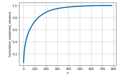
From the above diagram, 20% of the information is explained when converted to 10-D. If 784-D trasnformed to 300-D, alomst 95% of the information is retained.
2D visualization of MNIST Data
Let’s visualize the 784-D MNIST dataset in 2-D to get a clear understanding of PCA.
First, covariance matrix will be calculated by multiplying the data with the transpose of same data. co-variance(S) = xT*x
# Constructing a co-variance matrix
covar_matrix = np.matmul(data.T,data)
Then, eigen values and eigen vectors are formulated from the co-variance matrix using eigh function imported from scipy.linalg. As the top 2 valued eigen values and vectors are needed for 2-d and these values will be arranged in ascending order, we would consider only 782 and 783 values.
# Finding the top 2 eigen values and vectors
# As the eigen values and vectors are arranged in ascending order, take last 2 values.
from scipy.linalg import eigh
values, vectors = eigh(covar_matrix, eigvals=(782,783))
vectors=vectors.T
Finally, the new data with 2 dimensions will be obtained by multiplying the vectors matrix with the original data and the labels will be stacked with the new data, indicating the size (20000,3).
coordinates=np.matmul(vectors,data.T)
coordinates = np.vstack((coordinates, labels)).T
new_data=pd.DataFrame(data=coordinates, columns=("1st_principal_axis", "2nd_principal_axis", "label"))
sns.FacetGrid(new_data,hue="label",height=6).map(plt.scatter,'1st_principal_axis','2nd_principal_axis').add_legend()
plt.show()
2-D visualization
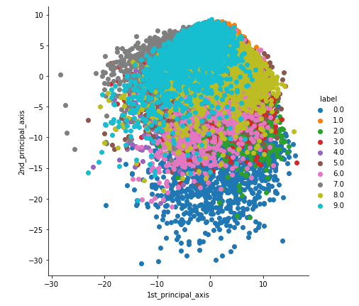
From the figure, one cannot differentiate the numbers as only 10% of the information is explained in 2-D.